Introduction
Ledge is a rebalancing execution engine for factor risk models, written in Rust with first-class Python bindings.
It solves continuous convex mean-variance portfolio QPs whose covariance has factor structure
\[ \Sigma = F \Omega F^\mathsf{T} + \mathrm{diag}(d) \]
without ever forming the dense \(n \times n\) matrix. Inputs are the factor loadings \(F\), the factor covariance \(\Omega\), idiosyncratic variances \(d\), expected returns \(\mu\), constraints, and previous weights. Outputs are auditable weights (independent KKT residuals), duals, and diagnostics.
What it covers
- Mean-variance objectives with budget, weight boxes, linear equality and inequality constraints.
- Smooth L2 turnover and exact L1 proportional transaction costs with a machine-exact no-trade region.
- Tracking-error objectives against a benchmark.
- Constraint templates: industry neutrality, group targets, style bands, concentration and short limits.
- Rolling sequences with automatic warm starts and factorization reuse, and multi-threaded batch over many accounts.
- Trust machinery on by default: automatic scaling, audit-gated solution polishing, infeasibility certificates, and independent KKT checks on the original (unscaled) data.
What it deliberately does not cover
No mixed-integer constraints, no SOCP or general NLP, no GPU/distributed execution, and no alpha or risk-model estimation — \(F\), \(\Omega\), \(d\) are inputs. If you need a general modeling language, keep cvxpy; migrate only the rebalancing QP.
Declared envelope
Default settings are tested to converge on continuous convex factor QPs with roughly \(n \le 5000\) assets, \(k \le 100\) factors, and \(m \le 200\) explicit linear constraint rows. Outside that envelope Ledge may still work, but the project makes no default-settings promise.
Status
Alpha (0.2.x). APIs and defaults may change before 1.0; every change is
recorded in the repository
CHANGELOG. Source is
licensed Apache-2.0. Release 0.2.0 is available from
PyPI and
crates.io; see
Installation for package names and platforms.
Visual tour
From APIs to the numerical core
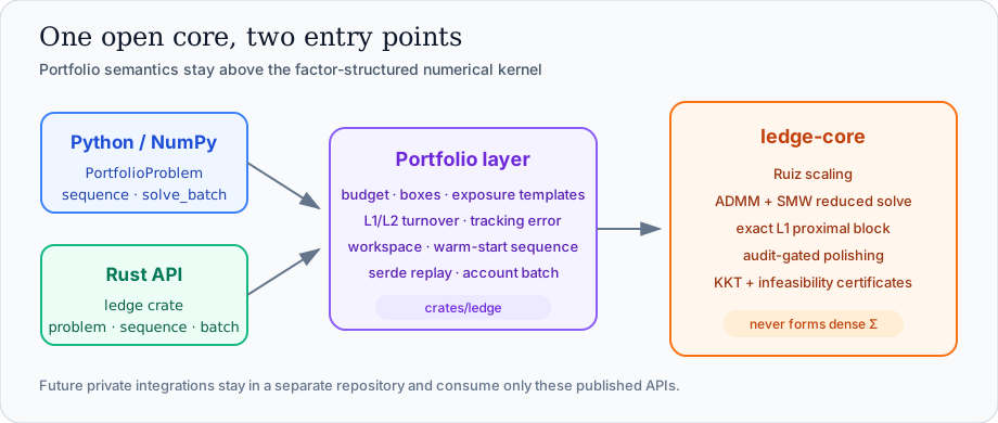
Python and Rust callers use the same portfolio semantics. The portfolio layer
compiles budget, boxes, exposure templates, turnover, and tracking error into
the factor-structured kernel. ledge-core performs scaling, ADMM/SMW updates,
the exact L1 proximal step, polishing, and independent audits without forming
the dense covariance matrix.
One model, many rebalance dates
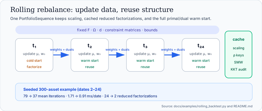
A PortfolioSequence holds fixed covariance and constraint structure. Each
date updates expected returns and holdings, then reuses cached reduced
factorizations and the preceding primal/dual solution. The annotation comes
from the repository's seeded 300-asset, 24-date example; run
python docs/examples/rolling_backtest.py to reproduce it.
Measured comparison, not a marketing sketch
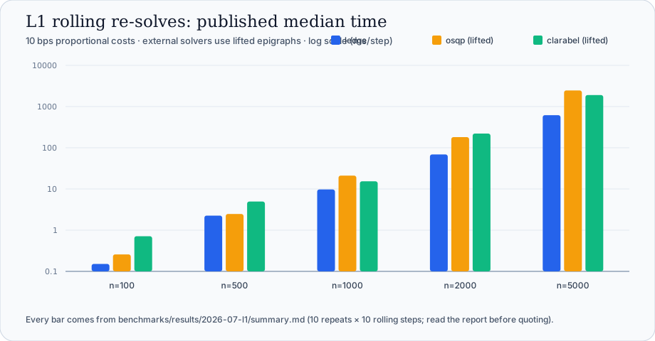
The bars are parsed directly from the committed
benchmarks/results/2026-07-l1/summary.md: ten repeats with ten rolling steps
per repeat. Ledge uses its native L1 proximal block; OSQP and Clarabel receive
factor-lifted epigraph formulations. The chart is deliberately logarithmic
because the range spans four orders of magnitude.
The full report includes setup, cold, rolling, status, iteration, and independently audited residual data. Read the benchmark evidence chapter before quoting a result.
Reproduce the visuals
From the repository root:
python scripts/generate_demo_assets.py --check
python scripts/generate_demo_assets.py
The script uses the standard library for SVGs and Pillow for the README's
terminal GIF. Provenance and refresh instructions live in
docs/assets/README.md.
Installation
Requirements: Rust 1.83+; Python 3.9+ for the bindings. There are no native dependencies (no BLAS/LAPACK) in the default build.
Rust
[dependencies]
ledge = { package = "ledge-portfolio", version = "0.2" }
Optional cargo features on ledge / ledge-core:
| Feature | Adds |
|---|---|
serde | Serialize/Deserialize for problems, settings, warm starts, and solutions |
rayon | multi-threaded solve_batch over the account axis (same API and identical results without it) |
Python
Install the published 0.2.0 release:
python -m pip install ledge-portfolio==0.2.0
Or build from source with maturin:
git clone https://github.com/Jiangki/ledge.git
cd ledge
python3 -m venv .venv
source .venv/bin/activate
python -m pip install --upgrade pip maturin
python -m pip install -e python/
python python/examples/rebalance.py
The Python package is named ledge-portfolio and imports as ledge. The
only runtime dependency is NumPy. The wheel enables the serde and rayon
features, so to_json / from_json and parallel solve_batch work out of
the box.
Verify the installation
cargo test --workspace          # Rust test suite
python -m pip install -e "python/[test]"
python -m pytest python/tests -q   # includes cvxpy+Clarabel gold tests
First solve (Python)
A minimal long-only mean-variance rebalance. Arrays must be NumPy float64.
import numpy as np
from ledge import PortfolioProblem

rng = np.random.default_rng(7)
n, k = 100, 8
F = rng.normal(0.0, 0.2, size=(n, k))       # factor loadings
omega = np.diag(rng.uniform(0.04, 0.12, size=k))  # factor covariance
d = rng.uniform(0.05, 0.10, size=n)         # idiosyncratic variance
mu = rng.normal(0.08, 0.02, size=n)         # expected returns

problem = PortfolioProblem(
    F,
    omega,
    d,
    mu,
    risk_aversion=8.0,
    budget=1.0,
    lower_bounds=np.zeros(n),
    upper_bounds=np.full(n, 0.03),
)
result = problem.solve()
print(result.status, result.weights.sum(), result.primal_residual)
The objective minimized is
risk_aversion / 2 * (w - b)' Sigma (w - b)      [b = 0 without a benchmark]
- expected_returns' w
+ turnover_penalty / 2 * ||w - previous_weights||^2
+ l1_turnover_costs' |w - previous_weights|
subject to sum(w) = budget, lower <= w <= upper, and any linear
constraints you pass (equality_matrix @ w = equality_rhs,
inequality_matrix @ w <= inequality_rhs).
The next date
Pass the previous solution as a warm start and price turnover:
next_problem = PortfolioProblem(
    F,
    omega,
    d,
    mu + rng.normal(0.0, 0.005, size=n),
    risk_aversion=8.0,
    lower_bounds=np.zeros(n),
    upper_bounds=np.full(n, 0.03),
    previous_weights=result.weights,
    l1_turnover_costs=0.001,   # 10 bps per unit traded; scalar broadcasts
)
second = next_problem.solve(warm_start=result.weights)
print(second)
For repeated dates prefer a rolling sequence, which caches the factorization and chains full primal/dual warm starts automatically.
Reading the result
SolveResult carries status, weights, objective, iterations,
solve_time_seconds, independently evaluated primal_residual /
dual_residual, polished, and — for infeasible problems — an auditable
certificate. The lossless to_json() output also contains every dual
multiplier block. Failures raise by default; pass raise_on_failure=False
to inspect the result instead. convergence_hints explains unconverged
solves in portfolio vocabulary.
One-shot function form: ledge.solve_mean_variance_factor(...) takes the
same keyword arguments and returns the same SolveResult.
First solve (Rust)
use ledge::{FactorCovariance, Matrix, PortfolioProblem, SolveStatus};

fn main() -> Result<(), Box<dyn std::error::Error>> {
    // 3 assets, 1 factor.
    let factors = Matrix::new(3, 1, vec![1.0, -0.5, 0.25])?;
    let problem = PortfolioProblem::new(
        factors,
        FactorCovariance::Diagonal(vec![0.1]),
        vec![0.2, 0.3, 0.25],   // idiosyncratic variances d
        vec![0.08, 0.04, 0.06], // expected returns mu
    )?
    .with_risk_aversion(5.0)?
    .with_bounds(vec![0.0; 3], vec![0.6; 3])?;

    let solution = problem.solve(None)?;
    assert_eq!(solution.status, SolveStatus::Solved);
    println!("{:?}", solution.x);
    Ok(())
}
PortfolioProblem is a builder; each with_* method validates eagerly so
mistakes fail at build time, not as mysterious infeasible solves:
| Builder | Adds |
|---|---|
with_risk_aversion, with_budget | objective scale and budget row |
with_bounds | per-asset boxes |
with_equalities, with_inequalities | explicit linear constraints (replace semantics — call before templates) |
with_turnover_penalty | smooth L2 turnover around previous weights |
with_l1_turnover | exact proportional transaction costs (prox block) |
with_tracking_benchmark | tracking-error risk term |
with_industry_neutrality, with_group_targets, with_style_bounds, with_concentration_limit, with_short_limit | constraint templates |
problem.solve(None) uses default settings; pass
Some(&solver) with a configured Solver for
custom settings, and
solution.warm_start() to seed the next solve with the full primal/dual
state.
The lower-level QpProblem API remains available for custom continuous
convex QPs with the same factor-structured quadratic.
Rolling rebalances
Rolling workloads — daily or weekly rebalances where mostly the expected
returns and the previous holdings change — are the workload Ledge is built
around. A PortfolioSequence keeps the Ruiz equilibration and the reduced
factorizations cached across dates and chains full primal/dual warm starts
automatically.

Python
sequence = problem.sequence()          # solver kwargs accepted here
for date in dates:
    result = sequence.solve_next(
        expected_returns=mu[date],
        previous_weights=held,         # turnover anchor for L2 and L1
    )
    held = result.weights
solve_next accepts only factorization-preserving updates:
| Keyword | Rolls |
|---|---|
expected_returns | the linear cost |
previous_weights | the L2/L1 turnover anchor |
benchmark_weights | the tracking benchmark (base problem must have one) |
budget | the budget row RHS |
equality_rhs, inequality_rhs | constraint right-hand sides (including template targets) |
Structural changes — covariance, constraint matrices, bounds, turnover penalty — are rejected with an explanatory error: build a new problem and a new sequence. This makes the cost model visible in the API: everything a step can express reuses the cached factorization.
Steps are atomic. A rejected date (bad feed, impossible budget) leaves the
sequence exactly as it was, so production loops can skip it and keep
rolling. An unconverged date (MaxIterations) does not abort the sequence;
an infeasible date restarts the next date cold so diverged duals never
poison the warm start.
Rust
let mut sequence = problem.sequence()?; // or sequence_with(&solver)
for step in steps {
    let solution = sequence.solve_next(&step)?; // step: RebalanceStep
}
// One-call form over a precomputed step list:
let solutions = ledge::solve_sequence(&problem, &settings, &steps)?;
Measured effect
From the repository's seeded momentum backtest (300 assets, 12 factors, 24
monthly dates, 10 bps L1 costs, tracking benchmark; see
docs/examples/README.md in the repository): warm dates converge in 37
iterations vs 79 cold (2.1x), 0.91 ms vs 1.71 ms (1.9x), and factorizations
drop from 24 to 2 across the backtest. Rolling steps reach a steady state of
zero refactorizations because revisited penalties hit the workspace
cache.
Many accounts: batch
solve_batch runs one rolling sequence per account, in parallel over the
account axis. Accounts share no state, so results are bit-identical to a
serial loop regardless of thread count — threading changes wall-clock,
never answers.
Python
import ledge

results = ledge.solve_batch(
    problems,                     # list[PortfolioProblem], one per account
    steps,                        # list[list[dict]]: per-account, per-date
    chain_previous_weights=True,  # backtest convention, see below
)
for account_result in results:    # input order preserved
    for solution in account_result:
        ...
Each step dict mirrors solve_next keyword arguments
({"expected_returns": ..., "budget": ...}). The GIL is released for the
whole batch.
chain_previous_weights=Trueimplements the backtest convention: after aSolveddate the turnover anchor moves to that date's solved weights; non-Solveddates leave the anchor unchanged (the account did not trade). An explicitprevious_weightsin a step wins. Requires a turnover term.- Failures stay per account: one account's bad feed never discards the other accounts' finished results. Errors name the account (and step) index.
Rust
use ledge::{solve_batch, BatchAccount};

let accounts: Vec<BatchAccount> = ...; // problem + ordered RebalanceSteps
let results = solve_batch(&accounts, &settings);
// Vec<Result<Vec<Solution>, PortfolioError>>, input order
Threading is behind the non-default rayon cargo feature (the Python
wheel enables it). Without the feature the same API runs serially with
identical results. RAYON_NUM_THREADS or a caller-installed pool controls
the width.
Published throughput
1 model × 500 accounts × 250 dates (n=200, k=15, L2+L1 turnover, chained
anchors): 12.9 s wall on 4 vCPUs — 9.7k account-date solves per second,
4.0x over the serial build, all 125k solves Solved. Raw samples and
methodology: benchmarks/results/2026-07-batch/ in the repository.
Constraints and templates
Native constraint blocks
Every problem has, in QP terms:
- one budget equality
sum(w) = budget; - per-asset boxes
lower <= w <= upper; - optional equality rows
A_eq @ w = b_eq; - optional upper inequality rows
A_in @ w <= b_in.
Rows are cheap but not free: the reduced factorization Ledge solves each
iteration has dimension r = factors + explicit rows, so a formulation
with O(n) explicit rows forfeits the factor-structure advantage. Boxes
are handled by a dedicated projection and never grow r.
Templates
Template builders compile portfolio vocabulary onto those blocks, with eager validation (empty groups, crossing bands, caps contradicting existing bounds fail at build time):
| Template (Rust / Python) | Compiles to |
|---|---|
with_industry_neutrality / industry_ids= | one equality row per industry, targets from the tracking benchmark |
with_group_targets / industry_ids= + industry_targets= | one equality row per group with explicit targets |
with_style_bounds / style_matrix=, style_lower=, style_upper= | inequality rows for the finite sides of each exposure band; exact bands collapse to one equality row |
with_concentration_limit / max_weight= | box tightening ` |
with_short_limit / max_short= | box tightening w_i >= -limit; 0 = long-only — no new rows |
Templates append to the user constraint blocks; with_equalities /
with_inequalities have replace semantics, so call those first. Appended
rows become ordinary user rows: rolling sequences move industry or style
targets date-by-date through equality_rhs / inequality_rhs step updates
with cached factorizations intact.
Python example
problem = PortfolioProblem(
    F, omega, d, mu,
    risk_aversion=8.0,
    lower_bounds=np.zeros(n),
    upper_bounds=np.full(n, 0.05),
    benchmark_weights=benchmark,
    industry_ids=industry_ids,        # industry-neutral vs the benchmark
    style_matrix=style_exposures,     # k_style x n
    style_lower=-0.1 * np.ones(k_style),
    style_upper=+0.1 * np.ones(k_style),
    max_weight=0.03,                  # concentration cap, box-only
    max_short=0.0,                    # long-only, box-only
)
A total short-budget cap (sum(max(-w, 0)) <= S) is deliberately not a
template: it needs a long/short variable split the QP form does not model.
Turnover and tracking error
Smooth L2 turnover
turnover_penalty (Python) / with_turnover_penalty (Rust) adds
\(\tfrac{\gamma}{2}\lVert w - w_0 \rVert^2\) around the previous weights.
It discourages trading everywhere but never produces exact no-trades. The
penalty sits on the diagonal of the quadratic, so changing it invalidates
cached factorizations — sequences therefore treat it as structure, not
data.
Exact L1 transaction costs
l1_turnover_costs (Python) / with_l1_turnover (Rust) adds proportional
costs \(\sum_i c_i \lvert w_i - w_{0,i} \rvert\) — a scalar broadcasts to
all assets. This is the term with a genuine no-trade region: assets
whose expected-return edge does not cover the round-trip cost stay exactly
at the anchor, machine-exact.
Implementation matters here. The standard epigraph reformulation adds n
auxiliary variables and 2n inequality rows, which destroys the
factor-structure advantage. Ledge instead handles the term as a dedicated
soft-threshold proximal block inside ADMM: the reduced factorization keeps
its factors + constraints dimension, and rolling sequences move the
anchor in O(n) without refactorizing.
The L1 multiplier is a first-class dual: the independent KKT audit scores the subgradient conditions (\(\lvert\lambda_i\rvert \le c_i\), with \(\lambda_i = \pm c_i\) on the trade sign when trading), polishing pins no-trade assets at the anchor, and warm starts carry the L1 dual. The implementation is validated against epigraph reformulations in Rust (including property tests) and against cvxpy+Clarabel in Python.
L2 and L1 can be combined; both use the same previous_weights anchor.
Tracking error
benchmark_weights (Python) / with_tracking_benchmark (Rust) turns the
risk term into active risk
\(\tfrac{\lambda}{2}(w-b)^\mathsf{T}\Sigma(w-b)\). Expanding the square
shows this is a pure linear-cost shift \(-\lambda\Sigma b\), computed
through the factor structure — the same QP underneath, no solver changes.
The constant \(\tfrac{\lambda}{2}b^\mathsf{T}\Sigma b\) is dropped from
reported objectives, as is conventional.
Because it is a linear-cost shift, sequences roll the benchmark
date-by-date (benchmark_weights in solve_next) with cached
factorizations intact. Industry-neutrality templates derive their targets
from the benchmark when one is present.
Hard turnover caps
Ledge prices turnover in the objective; it does not model a hard cap
norm1(w - w_prev) <= tau (that needs a variable split). If your process
requires cap semantics, keep cvxpy for those dates or tune the cost until
realized turnover sits where the cap did — see
Migrating from cvxpy.
Trust: audits, certificates, polishing
Ledge's policy is that you should never have to trust the solver's own claim of success. Every mechanism below evaluates on the original, unscaled problem data and is independently checkable.
Independent KKT audits
check_kkt recomputes primal and dual residuals from the returned point
and multipliers — including the L1 subgradient conditions — without using
any solver state. The reported primal_residual / dual_residual on every
solution come from this audit, never from internal scaled-space estimates.
The comparison harness applies the same audit to OSQP and Clarabel results,
so published cross-solver numbers use one referee.
Automatic scaling (default on)
Ten Ruiz equilibration passes balance the problem before iterating,
preserving factor structure (the scaling acts on rows of F and on d;
no dense matrix is formed). Scaling changes only the space ADMM iterates
in: termination and all reported residuals are evaluated on original data.
scaling_iterations=0 disables it.
Solution polishing (default on)
After convergence, the active set is guessed from the final iterate and one
direct KKT solve refines the solution — typically from ~1e-5 residuals to
1e-11 or better, for single-digit-percent extra time. The polished
candidate is adopted only if the audited worst KKT residual improves;
degenerate active sets are rejected and the ADMM iterate returned
unchanged, so polish never degrades a solution and never ships uncertified
multipliers. SolveResult.polished / Solution::polished records the
outcome.
Infeasibility certificates
Contradictory constraints do not burn 10 000 iterations. The solver detects
divergence directions and returns PrimalInfeasible (with a normalized
Farkas certificate) or DualInfeasible (with an unbounded descent ray).
Certificates are attached to the solution, auditable with
check_primal_certificate / check_dual_certificate, and translated into
portfolio vocabulary — e.g. "budget row conflicts with the sector caps" —
as the leading hint.
The default infeasibility_tolerance=1e-5 is deliberately stricter than
OSQP's, because a false "your portfolio is infeasible" is worse than a slow
MaxIterations: problems infeasible by a smaller margin fall back to
MaxIterations with hints.
In Python, infeasible statuses raise by default with the hint as the
message; pass raise_on_failure=False to inspect
SolveResult.certificate.
Unconverged solves
MaxIterations results carry convergence_hints: which residual
dominates, whether the penalty was re-tuned repeatedly, and what to try
(more iterations, scaling, looser tolerance). The final iterate is still
returned with honestly reported residuals.
Saving and replaying problems
Bug reports and regression tests need a lossless way to capture exactly
what the solver saw and returned. Ledge ships this behind the non-default
serde cargo feature (enabled in the Python wheel).
Python
dump = problem.to_json()          # lossless problem dump
restored = PortfolioProblem.from_json(dump)

result = problem.solve()
report = result.to_json()         # status, weights, duals, residuals,
                                  # diagnostics, certificates
Attach the two JSON strings to a bug report and the maintainer can replay your exact solve — round-trips are bit-exact, so the replayed problem produces the identical iterate path.
Rust
QpProblem, PortfolioProblem, SolverSettings, WarmStart, and
Solution implement Serialize/Deserialize with any serde format:
let json = serde_json::to_string(&problem)?;
let restored: PortfolioProblem = serde_json::from_str(&json)?;
Notes:
- Validation cannot be bypassed. Matrices rebuild through their
constructors and
PortfolioProblemreplays its builder methods, so a tampered dump fails with the same errors as wrong constructor input. - JSON and infinities. Unbounded box sides travel as
null(Option<f64>per entry) because JSON has no representation for infinities. Any self-describing binary serde format works unchanged. - Bit-exact JSON parsing requires
serde_json'sfloat_roundtripfeature (default parsing may be off by 1 ULP). - Solutions from
NumericalFailurecontain non-finite iterates and only round-trip through binary formats.
Migrating from cvxpy
A mapping from the cvxpy patterns used in factor-model portfolio
rebalancing to the Ledge Python API. Every code pair in this guide is
executed and cross-checked against cvxpy + Clarabel by
python/tests/test_migration_guide.py,
so the mappings stay correct as APIs evolve.
Ledge is not a cvxpy replacement. cvxpy is a modeling language over many solvers; Ledge is one specialized solver for one problem family. Migrate the rebalancing QP; keep cvxpy for everything else.
1. Should you migrate?
Migrate a workload when all of the following hold:
- The objective is mean-variance (optionally with tracking error, L2 turnover, and/or proportional transaction costs) and the constraints are linear: budget, weight boxes, exposure equalities, upper inequalities.
- The covariance already has factor structure
Sigma = F @ Omega @ F.T + np.diag(d)— Ledge takesF,Omega,ddirectly and never forms then x nmatrix. - Instances live inside the declared envelope: roughly
n <= 5000assets,k <= 100factors,m <= 200explicit linear constraint rows. - The workload is repeated: rolling backtests and daily rebalances are where
warm starts and factorization reuse pay (see the measured numbers in
docs/examples/README.md).
Stay in cvxpy when you need anything outside that set, for example:
- integer or cardinality constraints (
w != 0counting, buy-in thresholds); - second-order-cone or exponential-cone terms (robust epsilon-balls, CVaR with auxiliary formulations beyond a QP);
- objectives that are not a convex QP plus absolute-value terms;
- a hard turnover budget
cp.norm1(w - w_prev) <= tau. Ledge prices turnover in the objective (l1_turnover_costs) instead of capping it; if your process needs the cap semantics, keep cvxpy for those dates or tune the cost until realized turnover sits where the cap did.
2. The core model
Ledge minimizes, over weights w with sum(w) = budget and
lower <= w <= upper plus optional linear constraints:
risk_aversion / 2 * (w - b)' Sigma (w - b)   [b = 0 without a benchmark]
- expected_returns' w
+ turnover_penalty / 2 * ||w - previous_weights||^2
+ l1_turnover_costs' |w - previous_weights|
Two conventions to check before comparing numbers:
- Factor of 1/2 on the risk term. If your cvxpy model writes
gamma * cp.quad_form(w, Sigma)without the half, passrisk_aversion = 2 * gamma. - Maximization.
cp.Maximize(mu @ w - gamma/2 * cp.quad_form(...))is the same problem; Ledge's minimized objective is its negation. Compare weights, or evaluate one objective function of your own on both weight vectors (that is how Ledge's own gold tests avoid convention traps).
The basic long-only rebalance, side by side:
# cvxpy
w = cp.Variable(n)
Sigma = F @ Omega @ F.T + np.diag(d)          # dense n x n materialized
risk = 0.5 * gamma * cp.quad_form(w, cp.psd_wrap(Sigma))
prob = cp.Problem(
    cp.Minimize(risk - mu @ w),
    [cp.sum(w) == 1.0, w >= lower, w <= upper],
)
prob.solve(solver=cp.CLARABEL)
weights = w.value
# ledge
from ledge import solve_mean_variance_factor

result = solve_mean_variance_factor(
    F, Omega, d, mu,
    risk_aversion=gamma,
    budget=1.0,
    lower_bounds=lower,
    upper_bounds=upper,
)
weights = result.weights
Arrays are NumPy float64; Omega is passed as a dense PSD matrix (use
np.diag(...) for diagonal factor covariances). For repeated solves of one
structure, build a PortfolioProblem once instead of calling the one-shot
function (§6).
3. Constraint mapping
| cvxpy | Ledge |
|---|---|
cp.sum(w) == 1.0 | budget=1.0 |
w >= lower, w <= upper | lower_bounds=lower, upper_bounds=upper (pass together) |
A @ w == b (exposures, neutrality) | equality_matrix=A, equality_rhs=b |
A @ w <= b (caps) | inequality_matrix=A, inequality_rhs=b |
A @ w >= b (floors) | negate: rows -A, right-hand side -b |
l <= A @ w <= u | two stacked blocks: A with rhs u, -A with rhs -l |
| unconstrained budget | omit — but note Ledge always has a budget row; set it to the sum you want |
Floors and ranges, concretely:
# cvxpy: sector floors and caps
constraints += [S @ w >= floor, S @ w <= cap]

# ledge: one upper-inequality block
inequality_matrix = np.vstack([S, -S])
inequality_rhs = np.concatenate([cap, -floor])
There is no dedicated "sector constraint" type on either side: an
industry-neutral book, style bounds, or a concentration limit are all rows
of A. For the common templates Ledge builds those rows for you
(roadmap 3.1):
# cvxpy: industry weights pinned to the benchmark's, per-name cap
constraints += [S @ w == S @ b, w <= 0.06]

# ledge: template kwargs compile onto the same rows / boxes
result = solve_mean_variance_factor(
    F, Omega, d, mu,
    benchmark_weights=b,          # tracking objective ...
    industry_ids=industry_ids,    # ... and industry neutrality against b
    max_weight=0.06,              # box tightening, no extra rows
)
industry_ids is one integer per asset; add industry_targets= to pin
group weights explicitly (no benchmark needed). Style bands map through
style_matrix= / style_lower= / style_upper= (use ±np.inf for
one-sided bands), and max_short= caps per-name shorts (0.0 forces
long-only). Templates append to whatever equality_matrix /
inequality_matrix you passed, and their targets roll through
solve_next(equality_rhs=..., inequality_rhs=...) in sequences.
4. Turnover and transaction costs
# cvxpy
objective += 0.5 * eta * cp.sum_squares(w - w_prev)   # smooth L2 preference
objective += kappa @ cp.abs(w - w_prev)               # proportional costs
# ledge
result = solve_mean_variance_factor(
    F, Omega, d, mu,
    ...,
    previous_weights=w_prev,
    turnover_penalty=eta,        # L2; 0 to disable
    l1_turnover_costs=kappa,     # scalar broadcasts; per-asset array allowed
)
Both terms share the previous_weights anchor and can be combined. The L1
term is handled by a dedicated proximal block, not an epigraph
reformulation, so the no-trade region is machine-exact: assets whose
marginal utility change is below their cost stay exactly at
w_prev[i], which is what makes realized turnover reports clean. The L1
multipliers are audited in the KKT check like every other dual.
5. Tracking error
# cvxpy
active = w - benchmark
objective = 0.5 * gamma * cp.quad_form(active, cp.psd_wrap(Sigma)) - mu @ w
# ledge
result = solve_mean_variance_factor(
    F, Omega, d, mu,
    ...,
    benchmark_weights=benchmark,
)
One convention: Ledge drops the constant gamma/2 * b' Sigma b from the
reported objective (standard QP-solver behavior). Weights are unaffected;
add the constant back if you compare objective values directly.
6. Rolling backtests: cp.Parameter → PortfolioSequence
The cvxpy pattern for a rolling backtest keeps the problem and swaps parameter values so the solver can reuse its symbolic form:
# cvxpy
mu_parameter = cp.Parameter(n)
prob = cp.Problem(cp.Minimize(risk - mu_parameter @ w), constraints)
for date in dates:
    mu_parameter.value = mu_by_date[date]
    prob.solve(solver=cp.CLARABEL, warm_start=True)
Ledge's equivalent is a first-class object; it also chains full primal/dual warm starts and keeps the equilibration and reduced factorizations cached across dates:
# ledge
from ledge import PortfolioProblem

problem = PortfolioProblem(F, Omega, d, mu0, ..., previous_weights=w0,
                           l1_turnover_costs=0.001)
sequence = problem.sequence()
for date in dates:
    result = sequence.solve_next(
        expected_returns=mu_by_date[date],
        previous_weights=held_weights,      # rolls the turnover anchor
    )
    held_weights = result.weights
solve_next accepts only factorization-preserving updates: expected
returns, the turnover anchor, the tracking benchmark, the budget, and
equality / inequality right-hand sides. Changing the covariance, the
constraint matrices, bounds, or the penalty levels means the problem
structure changed — build a new PortfolioProblem and a new sequence
(cvxpy makes the same distinction: those are new cp.Problems, not
parameter updates). A rejected step leaves the sequence unchanged, so a bad
date can be skipped without restarting the backtest.
Measured effect on the repository's momentum-backtest example (300 assets,
12 factors, 24 dates): warm dates take 37 versus 79 iterations and 0.91 ms
versus 1.71 ms against per-date cold solves, with 24 factorizations
replaced by 2
(docs/examples/README.md).
7. Statuses, failures, and duals
| cvxpy | Ledge |
|---|---|
prob.status == cp.OPTIMAL | result.status == "solved" (default: anything else raises RuntimeError) |
cp.OPTIMAL_INACCURATE | closest is "max iterations" with convergence_hints |
cp.INFEASIBLE | "primal infeasible" + result.certificate (Farkas proof, checkable) |
cp.UNBOUNDED | "dual infeasible" + result.certificate.direction (descent ray) |
prob.value | result.objective (minimization convention, constants dropped per §5) |
constraint.dual_value | not exposed in Python yet; the Rust API returns all multipliers, and result reports independently audited KKT residuals |
Differences worth knowing:
- Some contradictions never reach the solver: impossible inputs that are
visible from the data alone (a budget outside what the boxes can sum to,
mismatched dimensions) raise
ValueErrorat build time, where cvxpy would returnINFEASIBLEafter a solve. - Ledge raises by default on anything other than
"solved". Passraise_on_failure=Falseto inspect the returned iterate,convergence_hints, andcertificateinstead — that is the mode to use inside backtest loops that skip bad dates. - Infeasibility errors name the conflicting constraints in portfolio vocabulary (budget vs caps vs bounds), and the certificate is a machine-checkable proof, not just a status.
result.primal_residual/dual_residualare always evaluated on your original data, never on internally scaled data, andresult.polishedreports whether the direct active-set refinement (residuals ~1e-11 instead of ~1e-5) was adopted.
8. Verify your migration
Do not trust either solver's reported objective when switching: evaluate
one NumPy objective of your own on both weight vectors, exactly like
python/tests/test_reference.py
and
python/tests/test_migration_guide.py
do:
def my_objective(weights):
    risk = 0.5 * gamma * weights @ (F @ (Omega @ (F.T @ weights))) \
         + 0.5 * gamma * weights @ (d * weights)
    return risk - mu @ weights   # + your turnover / tracking terms

assert my_objective(ledge_weights) <= my_objective(cvxpy_weights) + 1e-6
np.testing.assert_allclose(ledge_weights, cvxpy_weights, atol=1e-4)
Keep the cvxpy model in your test suite as an oracle for a few dates — that is cheap insurance and exactly how this repository guards its own solver.
Tuning solver settings
Defaults are chosen so that the declared envelope converges without tuning
— try defaults first. Every knob below exists in Rust
(SolverSettings) and as a Python keyword argument on solve(),
sequence(), and solve_batch().
| Setting (Python kwarg) | Default | Meaning |
|---|---|---|
max_iterations | 10_000 | ADMM iteration cap |
absolute_tolerance | 1e-6 | absolute stopping tolerance |
relative_tolerance | 1e-5 | relative stopping tolerance |
rho | 1.0 | initial augmented-Lagrangian penalty |
adaptive_rho | True | residual-balancing penalty adaptation |
over_relaxation | 1.6 | ADMM over-relaxation α ∈ (0, 2); 1.0 = plain ADMM |
scaling_iterations | 10 | Ruiz equilibration passes; 0 disables |
infeasibility_tolerance | 1e-5 | certificate detection threshold; 0 disables |
polish | True | audit-gated active-set refinement after Solved |
Rust additionally exposes sigma, check_termination_every,
adaptive_rho_interval / _tolerance / _multiplier, minimum_rho /
maximum_rho, and polish_regularization /
polish_refinement_iterations; see the SolverSettings rustdoc.
When something is slow or unconverged
Work through these in order:
- Read
convergence_hints. Unconverged results name the dominating residual and suggest the next step. - Check your formulation, not the solver. Explicit constraint rows
grow the reduced factorization (
r = factors + rows); prefer box constraints (max_weight,max_shorttemplates add no rows) and keepmin the low hundreds. - Warm-start rolling workloads through a sequence instead of solving cold each date — measured ~2x fewer iterations and zero steady-state refactorizations.
- Badly scaled data: leave
scaling_iterationson (it is the difference betweenSolvedandMaxIterationson ill-conditioned suites). If you disabled it for experiments, re-enable it. - Looser tolerance: for backtests,
absolute_tolerance=1e-5often halves iterations; polishing usually recovers accuracy afterwards (verifypolishedand the audited residuals). - More iterations: large
nwith tight boxes can legitimately need more than 10k iterations cold; warm-started dates will not.
What not to tune
over_relaxation: 1.6 measured 1.7–2.9x iteration cuts across the smoke matrix; per-instance tuning overfits.rho/ adaptation parameters: the residual-balancing policy replays the same penalty ladder every solve, which is what makes the factorization cache effective. Changing the ladder trades cache hits for guesses.polish=Falsebuys single-digit percent time and costs six orders of magnitude of residual accuracy.
API surface
Rust
Published API documentation:
ledge and
ledge-core.
To generate the Rust documentation locally:
cargo doc -p ledge-portfolio --no-deps --open
The ledge crate re-exports everything from ledge-core. Main types:
| Type / function | Role |
|---|---|
PortfolioProblem | portfolio-vocabulary builder over the QP |
QpProblem, FactorQuad, L1Term | the underlying factor-structured QP |
Solver, SolverSettings | settings container and entry point |
Solution, SolveStatus, DualVariables | results with audited residuals and duals |
Solver::workspace → Workspace | equilibration + factorization cache across solves |
PortfolioSequence, RebalanceStep, solve_sequence | rolling date-by-date API |
solve_batch, BatchAccount (feature rayon) | parallel multi-account batch |
check_kkt, check_primal_certificate, check_dual_certificate | independent audits |
generate_synthetic, SyntheticConfig | deterministic test instances |
Python
The package installs as ledge-portfolio, imports as ledge, and carries
docstrings on every public symbol:
import ledge
help(ledge.PortfolioProblem)
help(ledge.solve_batch)
| Symbol | Role |
|---|---|
ledge.PortfolioProblem | problem construction (NumPy arrays, keyword constraints/templates) |
.solve(**settings) | one solve → SolveResult |
.sequence(**settings) → PortfolioSequence.solve_next(...) | rolling API |
ledge.solve_batch(problems, steps, ...) | parallel multi-account batch |
ledge.solve_mean_variance_factor(...) | one-shot function form |
PortfolioProblem.to_json() / from_json(), SolveResult.to_json() | reproduction dumps |
SolveResult | weights, status, objective, audited residuals, diagnostics, certificate; to_json() includes the full dual blocks |
Python does not currently expose solution dual multipliers as direct
SolveResult attributes. Use to_json() when a bug report or audit needs
the complete serialized solver result.
Benchmarks and evidence
Ledge publishes measured, reproducible, protocol-compliant numbers and
nothing else. The protocol (benchmarks/README.md in the repository)
requires shared instance data, documented conversions, native statuses
verbatim, independent KKT re-verification of every returned point,
phase-split timing, and ≥10 repeats with all raw samples published.
The honest headline
- Dense-
Qusage of a general QP solver is 1–2 orders of magnitude slower than factor-aware solving. That gap is the cost of ignoring factor structure, measurable within the same external solver (dense vs lifted formulation). See the technical notedocs/factor_structure_note.md. - Ledge's comparative strength is rolling and turnover-aware workloads,
not universal cold-start speed. On instances with proportional (L1)
transaction costs — the realistic rebalancing case — Ledge is the
fastest solver at every size, cold and rolling, because the epigraph
reformulation external solvers need costs them 2–6x while Ledge's prox
block costs ~8%. On smooth instances a hand-lifted Clarabel formulation
remains the strongest cold baseline at
n >= 2000. - Ledge's audited residuals at defaults are
~1e-11or better since polishing; objectives across solvers agree once compared at comparable residuals.

This chart is generated from the committed 2026-07-l1 report. It is a
visual index, not a substitute for setup/cold/residual details in the report.
Published reports
All under benchmarks/results/ in the repository, each with raw samples:
| Report | What it measures |
|---|---|
2026-07/ | first protocol report (pre over-relaxation) |
2026-07-over-relaxation/ | re-run after α=1.6 became the default |
2026-07-workspace/ | re-run after factorization reuse across solves |
2026-07-l1/ | re-run with polish defaults + L1 turnover instances (prox block vs epigraph) |
2026-07-batch/ | 1 model × 500 accounts × 250 dates batch throughput |
Reproduce
# Self-timing smoke matrix (no external solvers):
cargo run -p ledge-portfolio --release --example synthetic -- --n 500 --k 10 --seed 42

# Full protocol comparison (OSQP + Clarabel behind non-default features):
cargo run --release -p ledge-bench-adapters --features osqp,clarabel \
  --bin compare -- --out /tmp/comparison --repeats 10 --rolling-steps 10

# Batch throughput:
cargo run -p ledge-portfolio --release --features rayon --example batch
Read each report's findings before quoting any single number; the reports state where external solvers win.
Design notes and roadmap
The canonical engineering documents live in the repository and stay there (single source of truth); this page is the map.
| Document | Content |
|---|---|
docs/PLAN.md | public technical plan: scope, architecture, quality, release policy |
docs/ROADMAP.md | executable milestones M0–M4 with exit criteria and technical notes |
docs/DECISIONS.md | decision log (ADR-style): what was chosen, why, what was rejected |
docs/OPEN_CORE.md | authoritative repository boundary and public-release runbook |
docs/algorithm.md | solver math: ADMM splitting, SMW reduction, scaling, certificates, polishing, L1 prox |
docs/factor_structure_note.md | short technical note: why factor structure is worth exploiting, with measured evidence |
docs/cvxpy_migration.md | cvxpy → Ledge mappings, executed in CI |
docs/SMOKE_TIMINGS.md | self-timing smoke matrix numbers |
Design pillars (short form)
- Never form Σ. The ADMM x-update solves through a Sherman–
Morrison–Woodbury reduction of dimension
r = factors + explicit rows; every feature (scaling, polishing, L1, templates) is designed to keeprsmall. - Trust before speed. Residuals are audited independently on original data; polish is adopted only when the audit improves; infeasibility claims carry checkable certificates; benchmark claims follow a written protocol with raw samples.
- Rolling is the product. Warm starts, the workspace factorization cache, sequences, and batch exist because rebalancing is a repeated solve, not a one-shot.
- Small dependency surface. Default builds have no BLAS/LAPACK, no
native dependencies;
serdeandrayonare opt-in features.
Milestone status
M0 (foundations), M1 engineering (scaling, over-relaxation, comparisons),
M2 (L1, certificates, polishing, workspace, sequences, tracking), and the
M3 engineering items (templates, batch, serialization, this docs site) are
complete; the public 0.2.0 crates, Python wheels, and documentation site
are live. Remaining roadmap items are adoption- and decision-driven:
external real workloads and the 1.0 compatibility review. Sparse F
support is deliberately deferred until a real workload needs it.